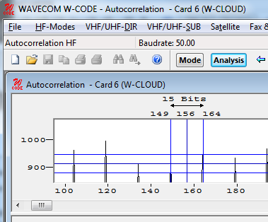
Autocorrelation is used for determining the periodicity of bit patterns. Periodicity implies a constant repetition of a specific bit pattern. If a station transmits the idle pattern 0010011011 0010011011..., the periodicity is said to be 10 bits. HNG-FEC and RUM-FEC have a periodicity of 15 and 16 bits respectively. The periodicity could also be 11250 bits, i.e., after 11250 bits the same constantly repeated pattern occurs again. Periodicity becomes very important in the classification of unknown transmissions and the analysis of unknown modes and systems.
First of all, the Auto option from the Demodulator menu field or the Auto button should be used to determine the exact baud rate and frequency shift. If the exact baud rate is unknown, the IAS measurement function can be used for this purpose with an accuracy of 0.001 Bd. This is done by activating the IAS setting in the Demodulator menu field. Autocorrelation is then initiated by selecting and programming the baud rate menu field. If the baud rate deviates by more than 0.5 Baud, a bit slip may occur and therefore the autocorrelation must be restarted with the exact baud rate.
To start the sampling process, press the Start button. The number of sampled bits is continuously displayed. Autocorrelation can currently process up to 200,000 bits.
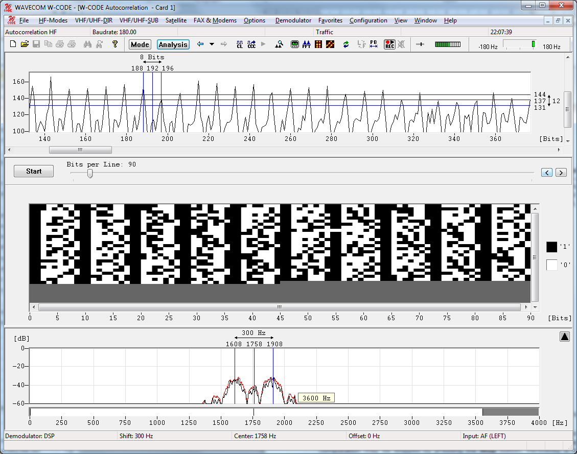
By pressing the Correlate button, the actual computation of the autocorrelation is started. Results are displayed graphically. If a large number of bits have been sampled and the graph indicates a low periodicity, the computation may be stopped by pressing the Stop button. Periodicity is indicated by distinct peaks in the graphic display, which may exhibit various characteristics:
Ø A large number of closely spaced vertical lines indicates a very small period (7 to 15 bits).
Ø Small and asymmetric peaks indicate that a distinct periodicity is not present. The presence of such small peaks may however be an indication of a very long period.
Ø In the case of a very "noisy" graph, periodicity cannot be determined without the zoom function. Such measurements indicate the fact that the system is transmitting data (traffic state). The user should then wait for an idle state or for some request (RQ) cycles for closer examination.
Ø The graphic display only shows approximate wave forms. This peculiarity is often evident in the case of simplex systems, however an approximate determination is still possible.
Ø In the case of a horizontal line without any peaks or deviations, no periodicity may be deduced, or the period is much larger than the total number of sampled data bits.
Each mode and each signal can produce very different displays. Often, it is possible to determine a periodicity with the zoom function.
For FSK signals the polarity is changed from the menu Options | Signal Polarity, and then using the buttons in the window shown. For more information see Signal Polarity.
For PSK signals the configuration of the symbol definition is in the menu Options | Symbol Definition. For more information see Symbol Definition.
By selecting Zoom In, the mouse cursor changes its shape. By clicking and dragging, a field can be enlarged or reduced horizontally and vertically. The field should be sized in such a way that the peaks fill out the zoom field optimally.
After the zoom field has been sized, release the mouse button. An enlarged section of the autocorrelation trace is displayed.
The distance between recurring, equidistant peaks gives the periodicity of the signal under investigation.
By selecting Zoom 100% the full screen display will reappear.
Several Color schemes are available through the right-click menu.